Stochastic Optimization · Generative AI · Decision Rules

Beyond Linear Decision Rules:
LLM-Guided Representation Discovery for Data-Driven Optimization

Generative Stochastic Optimization (GenSO): using LLMs to discover nonlinear recourse representations — without sacrificing rigor, tractability, or interpretability.

Huan Zhang, Yang Wang (Northwestern Polytechnical University) · Hanzhang Qin (National University of Singapore) · Yue Zhao (HSBC Business School, Peking University)

Conference Presentation · ~40 minutes

Agenda

Outline

1 · Problem & Motivation

The expressiveness–tractability tradeoff of decision rules, and the opportunity created by LLMs.

2 · Related Literature

Where GenSO sits across five streams of OR / ML research.

3 · The GenSO Framework

From LDR to Generative LDR; the LLM-guided evolutionary discovery loop.

4 · Theory: Finite-Sample & Search Bounds

Separating estimation error from search error; key insights.

5 · Numerical Studies

Multi-period inventory control & data-center location with real cloud traces.

6 · Takeaways

What LLMs should and should not do inside optimization.

01

Problem & Motivation

Why even an optimally-fitted linear decision rule can be far from optimal — and why this gap cannot be closed with more data.

Problem · 1 / 5

Decision-Making Under Uncertainty

Stochastic optimization with recourse: a here-and-now decision $\bm x$ is chosen before uncertainty $\tilde{\bm z}$ is revealed; a wait-and-see recourse $\bm y$ adapts after.

Central question: the decision maker commits to $\bm x$ before the outcome, then adapts $\bm y(\bm z)$ after — we want one deployable, expressive, yet tractable rule, not a separate solution per scenario.

$$\hat Z=\min_{\bm x\in\mathcal X}\ \mathbb E_{\hat{\mathbb P}}\!\left[\bm c(\tilde{\bm z})^\top\bm x+Q(\bm x,\tilde{\bm z})\right],\qquad Q(\bm x,\bm z)=\min_{\bm y}\big\{\bm d^\top\bm y:\ \bm A(\bm z)\bm x+\bm B\bm y\ge \bm b(\bm z)\big\}$$

Ideal: arbitrary policies

Recourse can be any measurable function $\bm y(\bm z)$ → maximal adaptivity, but generally intractable.

Reality: scenario SAA

SAA gives a separate $\bm y_s$ per training scenario — optimal in-sample, but not a deployable rule for unseen $\bm z$.

Problem · 2 / 5

The Tractability–Expressiveness Tradeoff

The dominant device is the Linear Decision Rule (LDR) — restrict recourse to be affine in the uncertainty:

$$\mathcal L^{N_z,N_y}=\Big\{\,\bm y:\ \bm y(\bm z)=\bm y_0+\textstyle\sum_{i\in[N_z]}\bm y_i\,z_i\,\Big\}$$

✓ Why it is used

Reduces an intractable adaptive problem to a finite LP
Small coefficient dimension
Interpretable & deployable

✗ The hidden cost

Strong inductive bias: recourse must vary linearly with $\bm z$
Cannot express thresholds, ratios, lags, peaks…

Classical rules trade off along a frontier; GenLDR pushes past it — yet stays below the intractable all-policies ceiling.

Oracle class & key point

$\mathcal R:=\{\bm y:\mathcal Z\to\mathbb R^{N_y}:\bm y\text{ is measurable and non-anticipative}\}$ is the unrestricted oracle class.

Key point: Even perfectly fitted LDR coefficients can remain far from optimal when the representation is too restrictive.

Problem · 3 / 5

An Irreducible Approximation Gap

First define the performance notation. For any deployed decision rule $\bm y$, let $\mathcal J(\bm x,\bm y)$ be its true out-of-sample expected cost.

$$Z^\star_{\mathcal R}:=\inf_{\bm x,\,\bm y\in\mathcal R}\mathcal J(\bm x,\bm y),\qquad Z^\star_{\Phi}:=\inf_{\bm x,\,\bm y\in\mathcal L_{\Phi}}\mathcal J(\bm x,\bm y)$$

Here $\mathcal R$ is the unrestricted oracle policy class, and $\mathcal L_\Phi$ is the decision-rule class induced by a fixed basis $\Phi$. Then the deployed cost decomposes as:

$$\underbrace{\mathcal J(\hat{\bm x},\hat{\bm y})-Z^\star_{\mathcal R}}_{\text{total gap to oracle}}=\underbrace{\mathcal J(\hat{\bm x},\hat{\bm y})-Z^\star_{\Phi}}_{\text{estimation error}\ \to 0\ \text{as }S\to\infty}\;+\;\underbrace{Z^\star_{\Phi}-Z^\star_{\mathcal R}}_{\text{representation gap}}$$

Estimation error

Vanishes with more data $S$. Classical statistical learning.

Representation gap

Does not vanish with data. Fixed once the basis $\Phi$ (e.g. raw LDR) is chosen.

More data lowers each curve, but a fixed basis plateaus above the oracle. GenSO lowers the plateau itself.

Implication

Good recourse often depends on nonlinear summaries — demand seasonality, workload imbalance, recent volatility, bottlenecks. To close the gap we must enrich the representation, not just collect more data.

Problem · 4 / 5

LLMs: An Opportunity — and a Trap

The opportunity

LLMs generate expressions, executable code, and problem-specific abstractions from textual + mathematical + domain context — exactly the nonlinear features that are hard to hand-design.

The trap: LLM as end-to-end solver

Hallucinations
No feasibility / optimality guarantees
Limited interpretability

The LLM only proposes the representation; it never chooses $\bm x$ or the coefficients $\bm y_h$.

Design principle

Use the LLM for what it is uniquely good at — proposing functional structure — and keep optimization for what it is uniquely good at: fitting, feasibility, and out-of-sample evaluation.

This separation of roles is the heart of the paper. The LLM never chooses $\bm x$ or the coefficients $\bm y_h$.

Problem · 5 / 5

Our Answer & Contributions

GenSO in one line

The LLM searches over representations; optimization fits coefficients. Recourse stays linear in fitted coefficients, but over LLM-generated basis functions.

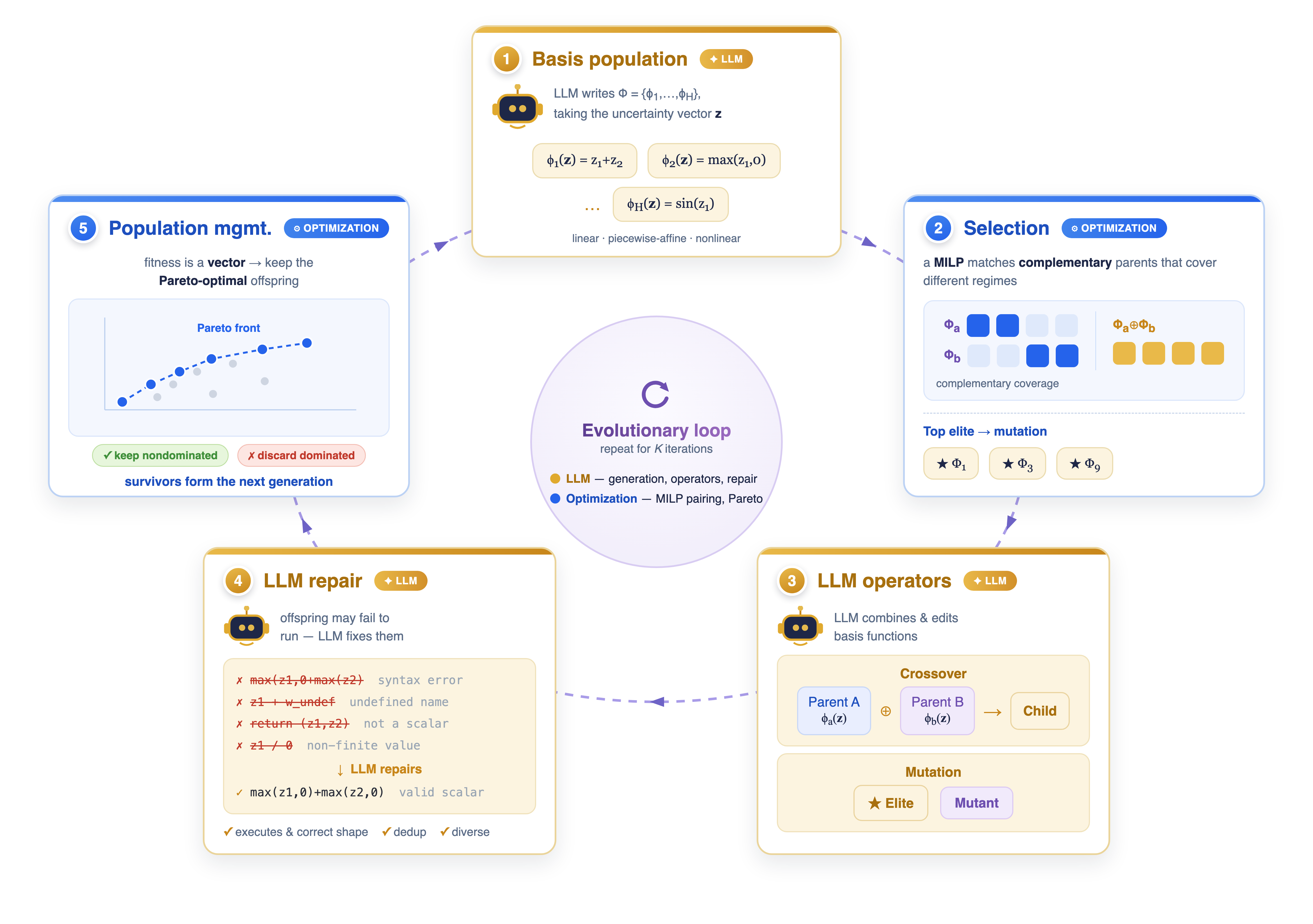
GenSO is a closed loop — generate → fit → validate → evolve — and the best basis is deployed.

① GenLDR

Generated representations generalize LDR while preserving tractability.

② GenSO framework

LLM-guided evolutionary search plus optimization-based validation.

③ Theory

Finite-sample fixed-basis bound plus LLM-search performance bound.

④ Evidence

Inventory control and data-center studies show OOS gains and interpretable structures.

02

Related Literature

Five streams — and how GenSO differs from each.

Literature · 1 / 4

Data-Driven Stochastic & Robust Optimization

Stochastic / SAA

Model uncertainty via a distribution; SAA replaces it with the empirical one — asymptotic & finite-sample guarantees.

Birge & Louveaux; Shapiro; Kleywegt et al.

Robust / Adjustable RO

Guard against all realizations in an uncertainty set; adjustable RO for adaptivity.

Ben-Tal et al.; Bertsimas & Sim

Distributionally Robust

Worst case over an ambiguity set (moment, conic, Wasserstein); robust satisficing.

Delage & Ye; Mohajerin Esfahani & Kuhn; Long et al.

Our relation

GenSO is compatible with all of these. For a fixed generated basis, basis values are lifted uncertain quantities; coefficients can be fit by SAA, robust, or DRO machinery — enriching recourse while keeping tractability and out-of-sample evaluation.

Literature · 2 / 4

Decision Rules & Operational Data Analytics

Decision rules in optimization

LDR (Ben-Tal et al. 2004); when affine rules are optimal (Bertsimas et al.; Georghiou et al.)
Deflected / segregated LDR (Chen et al.); polynomial rules (Bampou & Kuhn); piecewise-linear & primal-dual (Kuhn et al.)
Lifted uncertainty in adaptive DRO (Bertsimas et al. 2019); multi-deflected CARA (Chen et al. 2025)

ODA & prescriptive analytics

Operational statistics judged by decision value, not predictive accuracy (Feng et al.)
Covariate-to-decision prescriptions (Bertsimas & Kallus; Ban & Rudin)

The common limitation

In all of these, the transformation / lifting / basis is specified manually by the modeler. GenSO automates this representation-design step. ODA serves as a conceptual bridge: both judge data summaries by downstream decision value.

Literature · 3 / 4

LLM-Guided Function Search & LLMs in OR

LLM + evolutionary search

FunSearch (Romera-Paredes et al., Nature 2024): pair an LLM with an evaluator to discover new mathematical constructions / algorithms. Extended by EoH, ReEvo, AlphaEvolve, …

Mostly in CS/AI; LLMs generate complete programs.

LLMs in OR

Auto-formulation: NL → model (OptiMUS, ORLM, …)
Auto-modeling for robust / DP / SAA
LLMs as end-to-end combinatorial solvers
Operational apps: fleets, inventory; OM vision papers

Our positioning

We transfer the FunSearch idea to adaptive decision rules and redesign the search around mathematical optimization: the LLM searches for expressive representations, while coefficients come from an optimization model — not an end-to-end optimizer, not a replacement for modeling.

Literature · 4 / 4

Where GenSO Sits

Approach	Who designs the representation?	Tractable?	Guarantees?	Interpretable?
Classical LDR	Modeler (raw $z_i$)	Yes (LP)	Yes	Yes
Polynomial / PWL rules	Modeler (fixed family)	Yes, but dim. blows up	Yes	Medium
ODA / prescriptive	Modeler (hand-crafted stats)	Yes	Yes	Yes
LLM end-to-end solver	LLM (whole decision)	—	No	Low
GenSO (this work)	LLM proposes basis; opt. fits	Yes (LP/MILP)	Yes	Yes

The gap we fill

A method that gets the expressiveness of generative search while keeping the rigor, tractability, and interpretability of optimization.

03

The GenSO Framework

From the LDR to the Generative LDR, and the LLM-guided discovery loop that finds the basis.

Framework · 1 / 10

Stochastic Linear Optimization with Recourse

The backbone. Coefficient mappings are linear in $\bm z$ up to an intercept:

$$\bm A(\bm z)=\bm A_0+\sum_i \bm A_i z_i,\quad \bm b(\bm z)=\bm b_0+\sum_i \bm b_i z_i,\quad \bm c(\bm z)=\bm c_0+\sum_i \bm c_i z_i$$

With $S$ i.i.d. scenarios $\hat{\bm z}_1,\dots,\hat{\bm z}_S$, the SAA problem solves a separate recourse per scenario:

$$\hat Z=\min_{\bm x,\,\bm y_1,\dots,\bm y_S}\ \frac1S\sum_{s}\big[\bm c(\hat{\bm z}_s)^\top\bm x+\bm d^\top\bm y_s\big]\ \ \text{s.t.}\ \ \bm A(\hat{\bm z}_s)\bm x+\bm B\bm y_s\ge \bm b(\hat{\bm z}_s)\ \forall s$$

The deployment problem

Per-scenario $\bm y_s$ is optimal in-sample but is not a function of $\bm z$ → it cannot be applied to a new realization. We need a parametric rule.

Framework · 2 / 10

From LDR to Generative LDR

Linear Decision Rule

$$\bm y(\bm z)=\bm y_0+\sum_{i\in[N_z]}\bm y_i\,z_i$$

Linear in the raw uncertainty components.

Generative LDR

$$\bm y(\bm z)=\bm y_0+\sum_{h\in[H]}\bm y_h\,\phi_h(\bm z)$$

Linear in LLM-generated basis functions $\Phi=\{\phi_h\}$.

“Generative” = the source of the basis: produced by generative AI rather than specified by hand. Classical LDR is the special case $\phi_h(\bm z)=z_h,\ H=N_z$.

Crucial property

For any fixed $\Phi$, the SAA problem stays a linear program in $\bm x$ and $\{\bm y_h\}$ — basis values are just numerical inputs. Expressiveness ↑, tractability preserved.

Framework · 3 / 10

In-Sample Hierarchy

Proposition

For any basis set $\Phi\supseteq\{z_h\}_{h=1}^H$: $\ \mathcal L^{N_z,N_y}\subseteq\mathcal L_\Phi^{N_z,N_y}$, hence

$$\hat Z_{\mathcal R}\ \le\ \hat Z_\Phi\ \le\ \hat Z_{\mathcal L}\ \le\ \hat Z$$

Enriching the basis can only improve the in-sample objective — a deterministic consequence of feasibility.
This holds for any enrichment, regardless of basis quality. So in-sample improvement is not the interesting question.

The real challenge

Does the enriched rule generalize out-of-sample? Fitting $H+1$ coefficient vectors on $S$ scenarios introduces estimation error. This needs the statistical analysis in Section 4.

Framework · 4 / 10

LLM-Guided Representation Discovery

A closed evolutionary loop, repeated $K$ iterations. The LLM and the optimization model act in tandem, but with sharply separated roles:

LLM Representation generator

Writes, recombines, mutates, and repairs executable basis functions.

OPT Validation engine

Fits coefficients, checks feasibility, scores out-of-sample, selects parents, and manages the Pareto population.

$$\Phi^{(k)}=G_{\bm\theta}(\bm\pi^{(k)})=\{\phi_1^{(k)},\dots,\phi_H^{(k)}\}$$

Prompt as search state

The prompt $\bm\pi^{(k)}$ encodes the problem description, the required I/O format, and feedback from previously evaluated bases. The detailed algorithmic picture appears on the five-stage algorithm slide.

Framework · 5 / 10

Optimization-Based Validation

Given a generated basis $\Phi^{(k)}$, GenSO evaluates it in two steps:

(i) Fit coefficients by solving an LP (basis values are constants):

$$\hat Z_{\Phi^{(k)}}=\min_{\bm x,\{\bm y_h\}}\ \frac1S\sum_s\Big[\bm c(\hat{\bm z}_s)^\top\bm x+\bm d^\top\big(\bm y_0+\textstyle\sum_h\bm y_h\,\phi_h^{(k)}(\hat{\bm z}_s)\big)\Big]\ \ \text{s.t. constraints}\ \forall s$$

(ii) Score the fitted rule on a held-out validation set → vector-valued fitness returned as feedback.

LLM = generative operator

Explores functional forms not in any fixed dictionary; reaches transformations unreachable by coefficient optimization alone.

Optimization = evaluator

Feasibility, coefficient fitting, out-of-sample scoring, Pareto population management — all stay inside the rigorous model.

Framework · 6 / 10

The Five-Stage Evolutionary Algorithm

LLM-guided five-stage discovery loop — Gold = LLM generation/repair. Blue = optimization-based selection, fitting, and evaluation.

Basis population: each individual is a set of executable functions $\phi_h:\bm z\to\mathbb R$.
Selection: validation fitness identifies complementary parents.
LLM operators: recombine parents and mutate strong individuals by editing code.
Repair: invalid functions are fixed or discarded.
Management: retain non-dominated offspring and loop for $K$ iterations.

Why the picture matters

The LLM explores representation space, while optimization decides which representations survive.

Framework · 7 / 10

Why a MILP for Parent Selection?

Unlike scalar-fitness selection, GenSO keeps a vector fitness $\bm f_\Phi\in\mathbb R^{S_{\rm val}}$ — scenario-level performance is preserved. Parents are chosen by goal-programming MILP with three objectives:

Coverage

Minimize the gap between best fitness of selected parents and best of the whole population, across all validation scenarios.

Size control

Penalize deviation from target size $G_2$ — bounds the crossover prompt length.

Quality floor

Exclude consistently poor parents; threshold $G_3$ drifts from mean → best fitness over generations.

Effect

Selects parents that are good on different scenarios — pairing complementary strengths, so crossover can combine specialized basis functions rather than near-duplicates.

Framework · 8 / 10

Why LLM-Generated Representations?

Family	Strength	Limitation
Raw LDR	Small coeff. dim., tractable	Only linear in raw $\bm z$ → fixed approximation gap
Polynomial	Approximates smooth recourse	# monomials explodes with dimension & degree
Piecewise-linear	Great for thresholds	Regions/breakpoints must be chosen by analyst
GenSO basis	Problem-specific nonlinear summaries, mixed forms	No need to commit to one global family

The central merit

GenSO is a description-guided navigator between classical choices. It keeps the problem linear in fitted coefficients, while LLM-generated programs expand the recourse rule’s representational vocabulary.

Framework · 9 / 10

Extension to Multi-Stage Decision Rules

Decisions made sequentially; the rule at period $t$ may depend only on the observed history. Non-anticipativity is enforced by construction — every period-$t$ basis takes only $\bm z_{[t-1]}$:

$$\bm y_t(\bm z_{[t-1]})=\bm y_{t,0}+\sum_{h=1}^{H_t}\bm y_{t,h}\,\phi_{t,h}(\bm z_{[t-1]}),\qquad \bm\Phi=(\Phi_1,\dots,\Phi_T)$$

Period-specific bases

The LLM generates a different history-summary at each period — natural when the oracle rule needs different features over time.

Still an LP

For fixed $\bm\Phi$, all basis values are numerical inputs → the multi-stage SAA is a linear program in $\bm x$ and $\{\bm y_{t,h}\}$.

04

Theory: Finite-Sample & Search Bounds

Separating what is purely statistical from what depends on the LLM search.

Bounds · 1 / 10

The Analytical Challenge

The LLM enters the model in a non-standard way: it does not output the decision rule — it proposes basis functions over which an SAA problem fits coefficients.

✗ Naïve approach

Treat the entire LLM as a hypothesis class → would need Rademacher / VC / metric-entropy control over a black-box space of programs (prompts, decoding, proprietary training data). Intractable.

✓ Our strategy

Condition on the generated basis. Once $\Phi$ is fixed, the rule is linear in a finite $\bm w$ and the loss is linear → control fitting by a sub-Gaussian argument. The LLM appears only in the search term.

Bounds · 2 / 10

The Core Decomposition

$$\mathcal J(\hat{\bm x},\hat{\bm y})-Z^\star_{\mathcal R}=\underbrace{\mathcal J(\hat{\bm x},\hat{\bm y})-Z^\star_{\Phi}}_{\text{(A) coefficient estimation \& selection}}+\underbrace{Z^\star_{\Phi}-Z^\star_{\mathcal R}}_{\text{(B) representation approximation}}$$

(A) Statistical error

After the search fixes a representable class — pure SAA generalization. §3.1: a fixed-basis finite-sample bound.

(B) Structural error

How well the generated basis serves as a decision-relevant representation for the oracle. §3.2–3.3: $\epsilon$-good basis sets + LLM prior mass.

Benchmarks

$Z^\star_{\mathcal R}$: unrestricted measurable oracle. $Z^\star_\Phi$: best GenLDR with basis $\Phi$ under the true distribution. $\ Z^\star_{\mathcal R}\le Z^\star_\Phi\le Z^\star_{\mathcal L}$.

Bounds · 3 / 10

Fixed-Basis Setup: Exploiting Linearity

Stack the decision and define a feature-cost vector so the loss becomes a single inner product:

$$\bm w=(\bm x,\bm y_0,\dots,\bm y_H)\in\mathbb R^{N},\quad N=N_x+(H+1)N_y$$

$$\bm\xi(\bm z)=\big(\bm c(\bm z),\,\bm d,\,\phi_1(\bm z)\bm d,\dots,\phi_H(\bm z)\bm d\big),\qquad \ell(\bm w,\bm z)=\bm\xi(\bm z)^\top\bm w$$

Why this matters

The scenario cost is linear in $\bm w$. So uniform convergence reduces to controlling $\|\hat{\bm\xi}_S-\bar{\bm\xi}\|_2$ — concentration of a sample mean — with no global complexity measure of the LLM program class.

Bounds · 4 / 10

Assumptions (Fixed Basis)

(i) Bounded optimizers

Independent components of $\tilde{\bm z}$; stacked optimal coefficients satisfy $\|\bm w\|_2\le R_\Phi$.
Prevents the empirical optimizer from amplifying sampling noise with huge coefficients.

(ii) Bounded differences

$\bm\xi(\cdot)$ changes by at most $L_i$ when coordinate $i$ changes.
More targeted than a global Lipschitz assumption.

These define the sensitivity constant used in the finite-sample bound:

$$\sigma_\Phi=\tfrac12\Big[\textstyle\sum_i L_{\Phi,i}^2\Big]^{1/2}$$

By McDiarmid's inequality, bounded differences ⇒ every 1-D projection of $\bm\xi(\tilde{\bm z})-\mathbb E\bm\xi$ is sub-Gaussian with parameter $\le\sigma_\Phi$.

Bounds · 5 / 10

Proposition: Uniform Convergence

Proposition 1

Under the assumptions, for any fixed $\Phi$, with probability $\ge 1-\eta$:

$$\sup_{\|\bm w\|_2\le R_\Phi}\big|\mathcal J_\Phi(\bm w)-\hat{\mathcal J}_S(\bm w)\big|\ \le\ C R_\Phi\sigma_\Phi\sqrt{\tfrac{N+\log(1/\eta)}{S}}$$

Proof in three moves

1 · One direction

McDiarmid ⇒ each projection is sub-Gaussian; sample mean has parameter $\sigma/\sqrt S$.

2 · $\varepsilon$-net

Cover the sphere by a $1/2$-net of size $\le 5^{N}$; norm $\le 2\max_{\text{net}}|\bm u^\top\bm v|$.

3 · Union bound

Over the net → convert back to a Euclidean-norm bound.

Uniformity is essential: the SAA optimizer is selected after seeing the data.

Bounds · 6 / 10

Theorem 1: Finite-Sample Bound

Theorem 1

For a fixed basis $\Phi$, with probability $\ge 1-\eta$ over $S$ i.i.d. scenarios:

$$\mathcal J(\bmh{x}^\star,\bmh{y}^\star)\ \le\ Z^\star_\Phi+2C R_\Phi\sigma_\Phi\sqrt{\tfrac{N+\log(1/\eta)}{S}}$$

Proof: split into (I) generalization error + (II) optimizer bias; each $\le\epsilon_S$ on the same uniform-convergence event.

$\sigma$

Coordinatewise sensitivity of the cost/features.

$R_\Phi$

Size of the coefficient search region.

$N/S$

Fitted parameters per training scenario.

Crucially: no complexity measure of the LLM program class appears — only conditional, fixed-basis quantities.

Bounds · 7 / 10

$\epsilon$-Good Bases & the LLM as a Prior

A useful basis set is decision-relevant: its best GenLDR nearly matches the unrestricted recourse oracle. Define the $\epsilon$-good basis sets:

$$\mathcal A_\epsilon=\{\,\Phi:\ Z^\star_\Phi-Z^\star_{\mathcal R}\le\epsilon\,\}$$

A frozen LLM + prompt induces a distribution over executable bases, $\mathbb Q_{\bm\theta}(\cdot\mid\bm\pi)$ — a problem-conditioned prior over representations. Empirical scaling laws motivate:

$$D_{\rm KL}\big(\mathbb Q^\star\,\|\,\mathbb Q_{\bm\theta}\big)\le A|\bm\theta|^{-\alpha}\ \ \Longrightarrow\ \ \mathbb Q_{\bm\theta}\{\Phi\in\mathcal A_\epsilon\mid\bm\pi\}\ge\Big(c_\epsilon-\sqrt{\tfrac{A}{2|\bm\theta|^\alpha}}\Big)_+$$

(Pinsker's inequality.) Larger models place more mass on $\epsilon$-good representations.

Bounds · 8 / 10

Assumption: LLM Prior Mass / Hit Probability

Assumption (hit probability)

There exist $c_1,c_2,\alpha>0$ (independent of $K,S,\eta,\eta',|\bm\theta|$) such that each search round hits an $\epsilon$-good basis with probability

$$\mathrm{Pr}\big(\Phi^{(k)}\in\mathcal A_\epsilon\mid\mathcal H_{k-1}\big)\ \ge\ \rho_\theta(\epsilon,\bm\pi)=\big(c_1-c_2|\bm\theta|^{-\alpha/2}\big)_+$$

Conditional on history $\mathcal H_{k-1}$ → the evolutionary search may be adaptive; independence across rounds is not required.
$c_1$: intrinsic prompt-conditioned mass of $\epsilon$-good representations. Larger model ⇒ larger lower bound.
The Pinsker-linearized form of the scaling-law KL bound.

Bounds · 9 / 10

Theorem 2: Combined Estimation + Search Bound

Theorem 2

With probability $\ge 1-\eta-\eta'$ over both basis generation and coefficient fitting:

$$\mathcal J(\bmh{x}^\star_K,\bmh{y}^\star_K)-Z^\star_{\mathcal R}\ \le\ \underbrace{\epsilon}_{\text{approximation}}+\underbrace{C_1R\sigma\sqrt{\tfrac{N+\log K+\log(1/\eta)}{S}}}_{\text{estimation + selection}}+\underbrace{\tfrac{C_2}{\eta'}e^{-K(c_1-c_2|\bm\theta|^{-\alpha/2})_+}}_{\text{LLM search penalty}}$$

Term 1: $\epsilon$

Small when generated bases can nearly match the oracle.

Term 2: estimation

Selecting among $K$ bases adds only $\log K$.

Term 3: search

Decays exponentially in $K$; improves with model scale $|\bm\theta|$.

Proof: chain-rule miss bound $\Pr(M_K)\le e^{-K\rho}$ + Markov; intersect with the union-bounded fixed-basis event.

Bounds · 10 / 10

Key Insight: GenSO vs. a Fixed Basis

Fixed basis $\Phi_0$ (e.g. LDR)

$$\Delta_{\Phi_0}+C_1R_{\Phi_0}\sigma_{\Phi_0}\sqrt{\tfrac{N_0+\log(1/\eta)}{S}}$$

The structural gap $\Delta_{\Phi_0}$ is fixed — it can only improve through more data $S$.

GenSO

$$\epsilon+C_1R\sigma\sqrt{\tfrac{N+\log K+\log(1/\eta)}{S}}+\tfrac{C_2}{\eta'}e^{-K\rho_\theta}$$

Replaces the fixed gap by $\epsilon$ + an exponentially shrinking search penalty.

The tradeoff & the levers

GenSO can improve along three axes a fixed basis cannot: more search budget $K$, a larger model $|\bm\theta|$, and a better prompt (higher $\epsilon$-good mass). Multi-stage: search effort scales as $K\sum_t H_t$; estimation scales like $\sqrt{T(H+1)/S}$.

05

Numerical Studies

Multi-period inventory control (synthetic demand) & data-center location with real cloud workload traces.

Numerical · 1 / 6

Setup & Benchmarks

What we compare

SAA (no adaptation)
SAA / LDR (full prespecified rule)
DRO — mean–variance & Wasserstein ambiguity (RSOME)
GenSO (ours)

Protocol

Train / validation / large held-out test split
Metric: deployed decision-rule cost $\hat{\mathcal J}^{\rm Eval}$ + 95% CVaR
Generator: DeepSeek V4, $K=20$ iterations
Basis budget capped ($H_t\le 10$ / $\le 5$)
Infeasible recourse projected onto feasible region

ODA connection

ODA motivates the idea of decision-relevant operational statistics; we use it as an analogy, not as a separate experimental benchmark.

Evaluation philosophy

All rules are scored as they would be deployed — applying the trained non-anticipative rule on each test path using only observed history.

Numerical · 2 / 6

Case 1 — Multi-Period Inventory Control

Seasonal demand, $T=24$, $c_+\!=\!5,c_-\!=\!1$. Mean cost (lower is better); GenSO is best at every uncertainty level $\gamma$.

Method	γ=.025	γ=.05	γ=.10	γ=.20
SAA (No Adapt.)	918	1827	3615	7249
SAA (Full LDR)	587	1172	2352	4569
DRO (Mean–Var)	599	1198	2396	4794
DRO (Wasserstein)	599	1198	2396	4794
GenSO (Ours)	534	1069	2174	4389

Improvement

vs LDR: ~4–9%↓ · vs DRO: ~8–11%↓ · lowest mean and CVaR throughout.

inventory-control boxplot — Out-of-sample cost over 1,000 test scenarios (γ=0.025). GenSO: lower median, narrower spread.

Numerical · 3 / 6

Figure 3 — Sensitivity Validates the Bound

parameter sensitivity for K M S — Out-of-sample cost under γ=0.025 as search budget, population size, and sample size vary.

Theory prediction

Theorem 2 separates estimation and search:

$$\epsilon+C_1R\sigma\sqrt{\frac{N+\log K}{S}}+\frac{C_2}{\eta'}e^{-K\rho_\theta}$$

Increasing $K$: lowers the LLM search penalty exponentially, while adding only $\log K$ to estimation.
Increasing $M$: expands representation diversity and improves the chance of finding low-gap bases.
Increasing $S$: reduces coefficient-estimation error and stabilizes validation.

Empirical message

The cost curves move in the directions predicted by the bound: better search and more data both improve deployed performance.

Numerical · 4 / 6

Case 1 — What Did the LLM Discover?

The generated basis functions are interpretable representations, not arbitrary nonlinearities. Two representative examples from the main text:

① Seasonal deviation

$$\phi^{(1)}=\frac{d_{t-1}-d_t^*}{1000},\quad d_t^*=1000\Big(1+0.5\sin\frac{\pi(t-1)}{12}\Big)$$

Compares the most recent demand with the nominal seasonal level. Positive values signal stronger-than-expected demand; negative values signal weaker demand.

② Historical peak-demand indicator

$$\phi^{(2)}=\min\left\{1,\max\left(0,\frac{\max_{\tau \lt t}d_\tau-1200}{1000}\right)\right\}$$

Detects whether past demand has exceeded a high-demand threshold. The clipping maps the signal into $[0,1]$, avoiding overreaction to extreme outliers.

Key insight

The LLM discovers lagged demand, thresholds, clipping, scaling, and cyclical phase terms — structures hard to pre-commit to with one polynomial or PWL family.

Numerical · 5 / 6

Case 2 — Data Center Location + Job Scheduling

Joint here-and-now: which sites to open, capacity, demand-to-site assignment. Adaptive recourse: per-period capacity allocation with backlog & terminal outsourcing → a MILP per fixed basis.

Real-world calibration

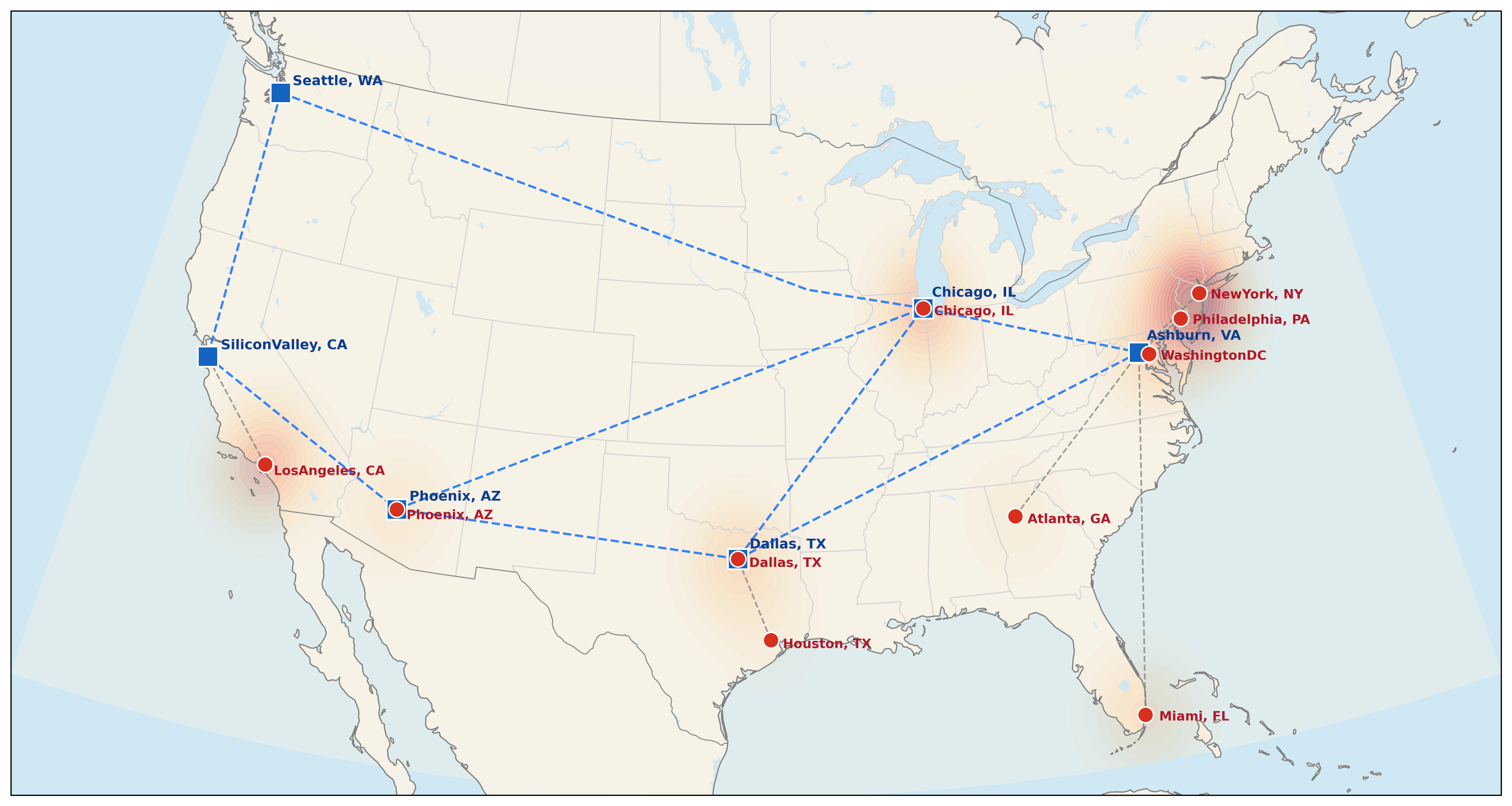
6 US data-center sites, 10 metro demand locations (PNNL IM3 Atlas)
Demand from Alibaba 2018 & Azure 2019 production traces
Costs calibrated to IM3 projections; dispatch ∝ geodesic distance
OOD test: train on Alibaba, also test on Microsoft

US data center demand map — Candidate data-center sites & metro demand locations.

Numerical · 6 / 6

Case 2 — Results & Out-of-Distribution Robustness

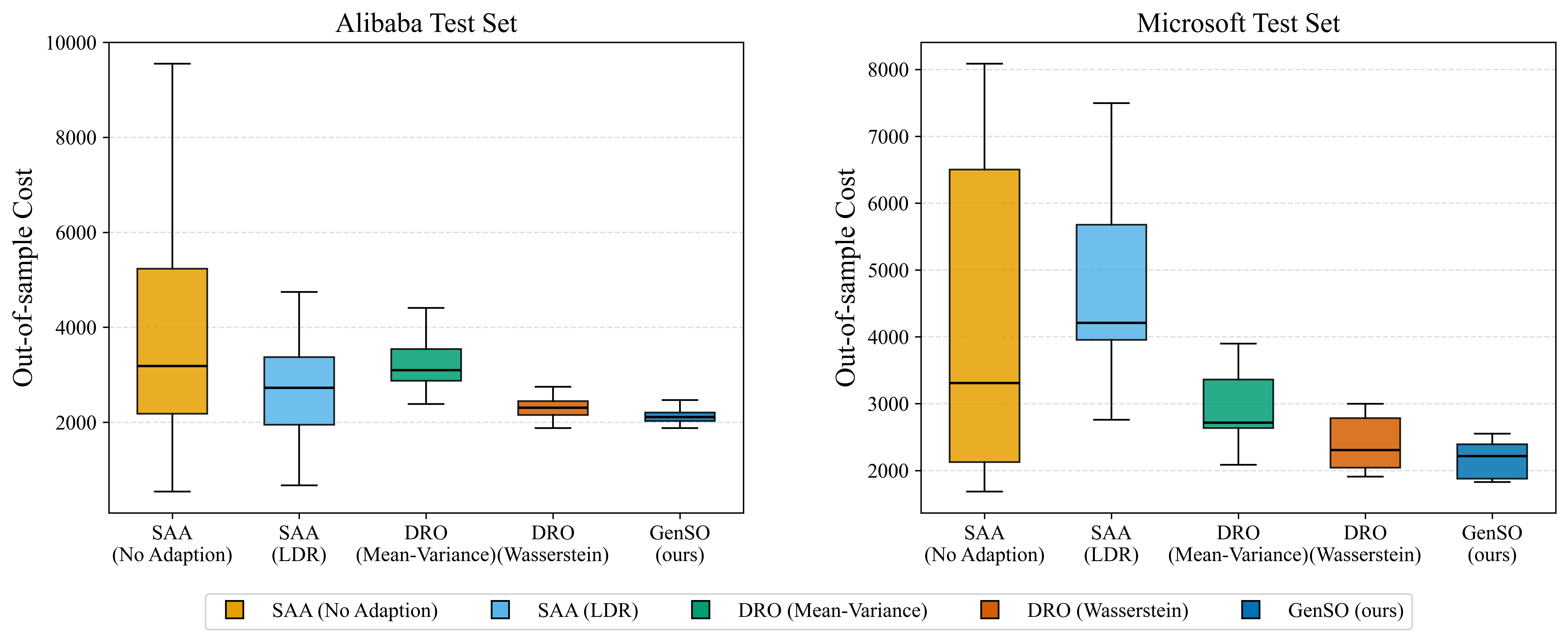
Multi-period $T=8$. Mean cost; lower is better. GenSO wins on both the in-distribution (Alibaba) and OOD (Microsoft) test sets.

Method	Alibaba	Microsoft (OOD)
SAA (No Adapt.)	3657	4132
SAA (LDR)	2658	4608
DRO (Mean–Var)	3208	2867
DRO (Wasserstein)	2304	2399
GenSO (Ours)	2123	2173

Generalization

vs LDR on OOD: ~53%↓. GenSO also has the smallest std & CVaR — the learned bases transfer to a different trace distribution.

two test sets boxplot — (a) Alibaba in-distribution (b) Microsoft out-of-distribution.

Numerical · Insights

What the Experiments Tell Us

Consistent wins

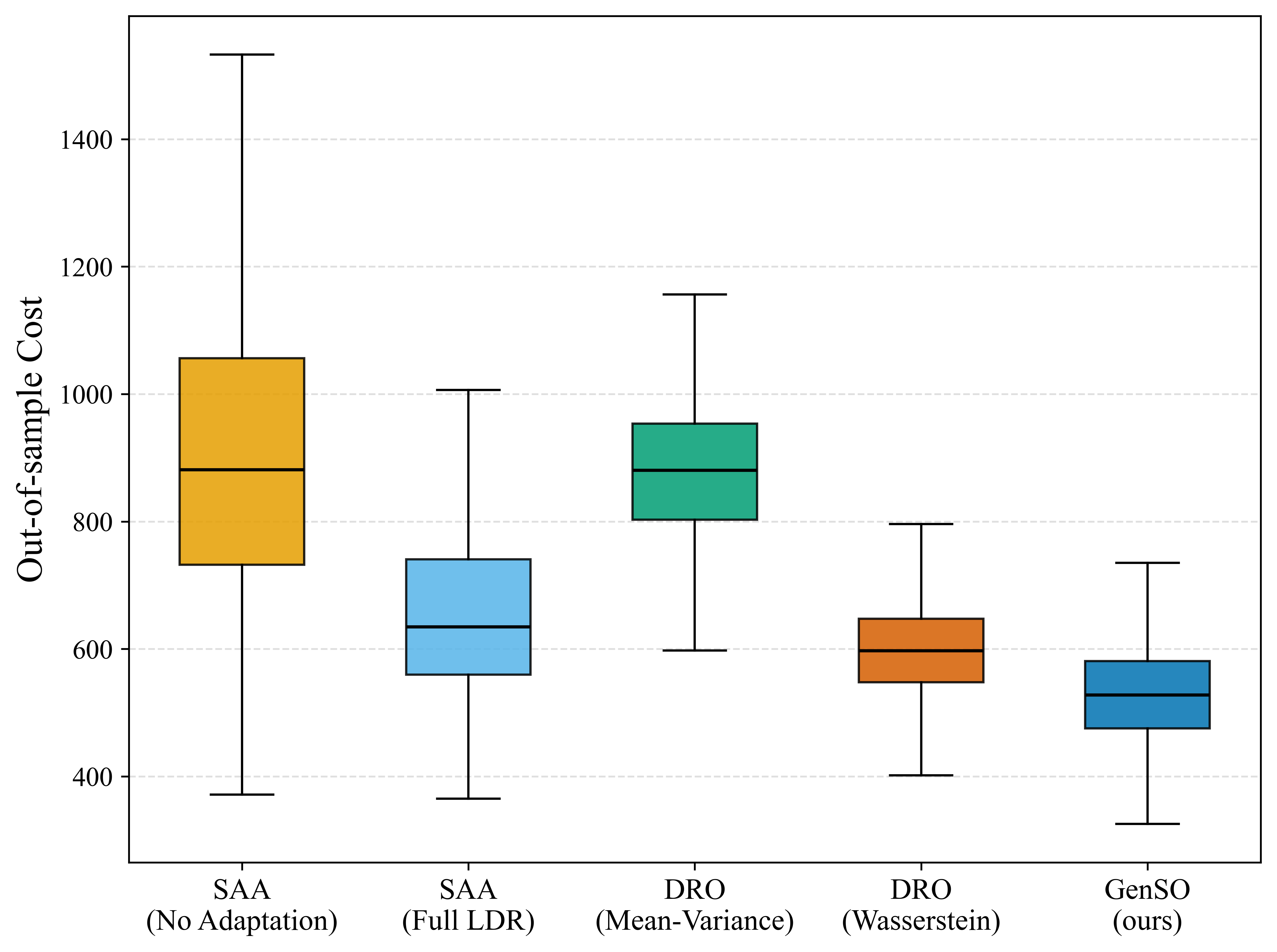
GenSO beats SAA, LDR, and both DRO variants on mean cost and CVaR, across uncertainty levels, horizons, and two domains.

Bound-aligned sensitivity

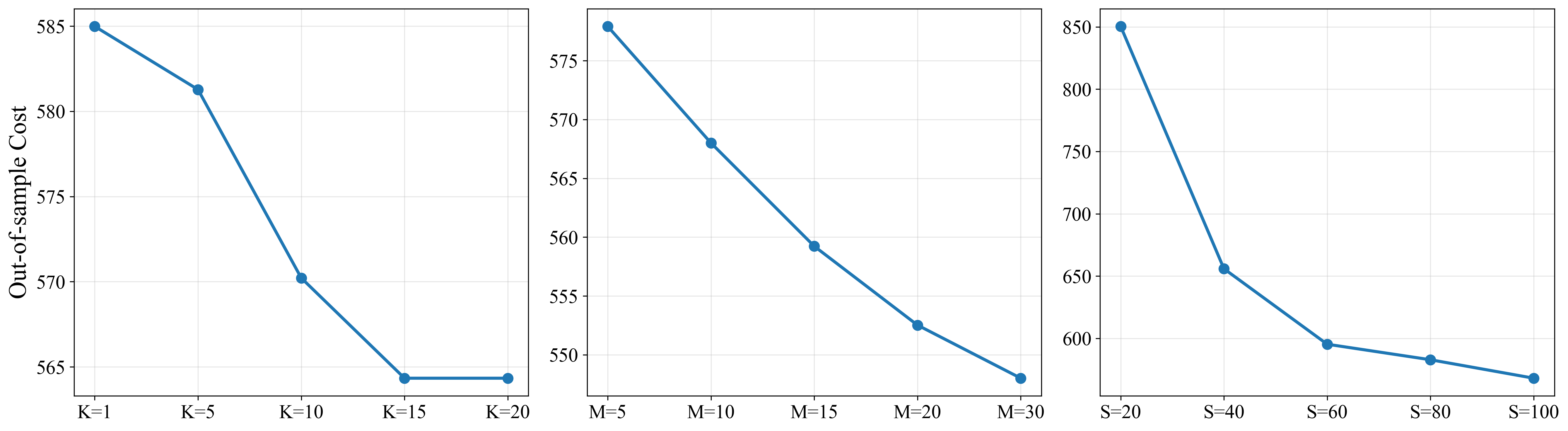
Figure 3 supports the theory: more search $K$, broader population $M$, and larger samples $S$ improve deployed cost.

Lower variance, better tails

Narrower out-of-sample spread → more reliable, not just lower on average.

Transfers out-of-distribution

Bases learned on Alibaba traces generalize to Azure — evidence they capture genuine operational structure.

Interpretability bonus

Discovered features (exponentially weighted moving averages, heteroskedasticity scaling, proximity-weighted network load, multi-scale cyclical patterns, backlog urgency) read like expert-designed operational statistics — but were found automatically.

Conclusion

Key Takeaways

① A new role for LLMs in OR

Not an end-to-end solver — a structured function generator inside a rigorous optimization model.

② GenLDR

Linear in fitted coefficients, but over LLM-generated nonlinear bases → expressiveness without losing tractability/interpretability.

③ Theory that separates concerns

Estimation error (classical SAA) + search error (exponential in $K$, improving with model scale) — no black-box complexity needed.

④ Real, transferable gains

Out-of-sample & out-of-distribution improvements with interpretable discovered structure.

Broader implication

The same recipe extends to pricing, revenue management, staffing, scheduling, transportation, and online optimization — anywhere good decisions depend on nonlinear summaries of history.

Thank You

Beyond Linear Decision Rules:
LLM-Guided Representation Discovery for Data-Driven Optimization

Questions & Discussion welcome

Huan Zhang · Yang Wang · Hanzhang Qin · Yue Zhao | NWPU · NUS · PKU

Approach	Who designs the representation?	Tractable?	Guarantees?	Interpretable?
Classical LDR	Modeler (raw \(z_i\))	Yes (LP)	Yes	Yes
Polynomial / PWL rules	Modeler (fixed family)	Yes, but dim. blows up	Yes	Medium
ODA / prescriptive	Modeler (hand-crafted stats)	Yes	Yes	Yes
LLM end-to-end solver	LLM (whole decision)	—	No	Low
GenSO (this work)	LLM proposes basis; opt. fits	Yes (LP/MILP)	Yes	Yes

Family	Strength	Limitation
Raw LDR	Small coeff. dim., tractable	Only linear in raw \(\bm z\) → fixed approximation gap
Polynomial	Approximates smooth recourse	# monomials explodes with dimension & degree
Piecewise-linear	Great for thresholds	Regions/breakpoints must be chosen by analyst
GenSO basis	Problem-specific nonlinear summaries, mixed forms	No need to commit to one global family

Beyond Linear Decision Rules:LLM-Guided Representation Discovery for Data-Driven Optimization

Agenda

Outline

1 · Problem & Motivation

2 · Related Literature

3 · The GenSO Framework

4 · Theory: Finite-Sample & Search Bounds

5 · Numerical Studies

6 · Takeaways

Problem & Motivation

Problem · 1 / 5

Decision-Making Under Uncertainty

Ideal: arbitrary policies

Reality: scenario SAA

Problem · 2 / 5

The Tractability–Expressiveness Tradeoff

✓ Why it is used

✗ The hidden cost

Problem · 3 / 5

An Irreducible Approximation Gap

Estimation error

Representation gap

Problem · 4 / 5

LLMs: An Opportunity — and a Trap

The opportunity

The trap: LLM as end-to-end solver

Problem · 5 / 5

Our Answer & Contributions

① GenLDR

② GenSO framework

③ Theory

④ Evidence

Related Literature

Literature · 1 / 4

Data-Driven Stochastic & Robust Optimization

Stochastic / SAA

Robust / Adjustable RO

Distributionally Robust

Literature · 2 / 4

Decision Rules & Operational Data Analytics

Decision rules in optimization

ODA & prescriptive analytics

Literature · 3 / 4

LLM-Guided Function Search & LLMs in OR

LLM + evolutionary search

LLMs in OR

Literature · 4 / 4

Where GenSO Sits

The GenSO Framework

Framework · 1 / 10

Stochastic Linear Optimization with Recourse

Framework · 2 / 10

From LDR to Generative LDR

Linear Decision Rule

Generative LDR

Framework · 3 / 10

In-Sample Hierarchy

Framework · 4 / 10

LLM-Guided Representation Discovery

LLM Representation generator

OPT Validation engine

Framework · 5 / 10

Optimization-Based Validation

LLM = generative operator

Optimization = evaluator

Framework · 6 / 10

The Five-Stage Evolutionary Algorithm

Framework · 7 / 10

Why a MILP for Parent Selection?

Coverage

Size control

Quality floor

Framework · 8 / 10

Why LLM-Generated Representations?

Framework · 9 / 10

Extension to Multi-Stage Decision Rules

Period-specific bases

Still an LP

Theory: Finite-Sample & Search Bounds

Bounds · 1 / 10

Beyond Linear Decision Rules:
LLM-Guided Representation Discovery for Data-Driven Optimization